Agriculture in East Asian Monsoon Area

Diverse forms of agriculture in Southeast Asia

Introduction

Southeast Asia is one of the regions where a wide range of agricultural practices has been carried out. Despite the overwhelming influence of the market economy, the tireless efforts of smallholder farmers over more than 1,000 years have created remarkably diverse array of farming systems. For example, in rice farming, which has long been the foundation of food security, farmers have developed numerous rice varieties, adaptive techniques to cope with erratic rainfall, fluctuations in crop prices, and, at times, strategies to escape the control of dominant political powers (Scott 2010). These farming techniques are well adapted to their local ecosystems and socioeconomic conditions.

While these agricultural practices have evolved in response to micro-landscape, much like the Darwinian evolution of living organisms, agricultural scientists have sought to construct overarching frameworks to explain farmers’ behaviors. Needless to say, socioeconomic factors such as food productions, crop market price, demographic dynamics (Boserup 1965) strongly influence these behaviors, but natural conditions also play a significant role in shaping farming practices over the long run.

Abundant natural resources and highly variable natural conditions are often considered as the two main factors shaping agriculture in this region. However, these two are frequently at odds. Interestingly, there is a clear divide among researchers: some emphasize environmental instability, while others highlight resource abundance. Researchers focusing on mainland Southeast Asia, such as Thailand, Laos, Myanmar, Vietnam, and Cambodia, tend to stress how farmers adapt to unstable and unpredictable natural conditions, especially precipitation (Fukui and Fukui 1993, Kono et al. 2012). On the other hand, scholars studying maritime Southeast Asia often emphasize the area’s rich biomass and high primary productivity (Tanaka 2010).

In this short essay, I aim to examine whether the instability or the abundance of natural resources has been the primary factor shaping agricultural systems in the long run, or whether both factors have played complementary roles. I also outline the methodological steps taken to approach this research questions.

East Asian Monsoon Area

The East Asian Monsoon region is unique in terms of its rainfall patterns (Kira 2012). Unlike other tropical and subtropical areas, it lacks arid zones. As a result, vegetation transitions continuously along temperature gradients, contributing to exceptionally rich biodiversity. This region also plays a vital role in agricultural production, making it and ideal context for comparing temperate and tropical farming systems.

Rather than focusing on meteorological perspectives, I aim to approach this topic from an agricultural standpoint to gain deeper insights into farming practices that sustains a significant portion of population.

Method

Load data

if (grepl("monsoon_asia", getwd())) {
    load(".RData")
} else {
    setwd("monsoon_asia/")
    load(".RData")
}

Load Library

library(tidyverse)
library(rgeoboundaries)
library(sf)
library(ncdf4)
# library(raster) duplication. The terra works instead of this.
library(terra)
library(rlang)
library(utils)
library(R.utils)
library(leaflet)
library(leaflet.extras)
library(htmlwidgets)
library(tmap)

Administrative Boundary

Visit geoBoundaries. Also see (Moraga and Baker 2022).

Show administrative boundary

se_asia <- c("THA", "LAO", "MYS", "IDN", "KHM", "MMR", "VNM", "TLS", "SGP", "BRN", "PHL")
e_asia <- c("PRK", "KOR", "JPN", "CHN", "MNG", "TWN")
east_monsoon <- c(se_asia, e_asia)

National border of Lao PDR

laos <- gb_adm0("LAO")
# laos <- geoboundaries("LAO")
plot(st_geometry(laos), graticule = TRUE, axes = TRUE)

# plot(laos$geometry, graticule = TRUE, axes = TRUE)

Provincial border

laos_prov <- gb_adm1("LAO")
plot(laos_prov$geometry, graticule = TRUE, axes = TRUE)

District border

laos_dis <- gb_adm2("LAO")
plot(laos_dis$geometry, graticule = TRUE, axes = TRUE)

National borders in East Asia

em_boundary <- gb_adm0(east_monsoon)

# Original data is too concise for the purpose, simplify the boundaries.

em_boundary_simp <- st_simplify(em_boundary, dTolerance = 0.01)
plot(st_geometry(em_boundary_simp))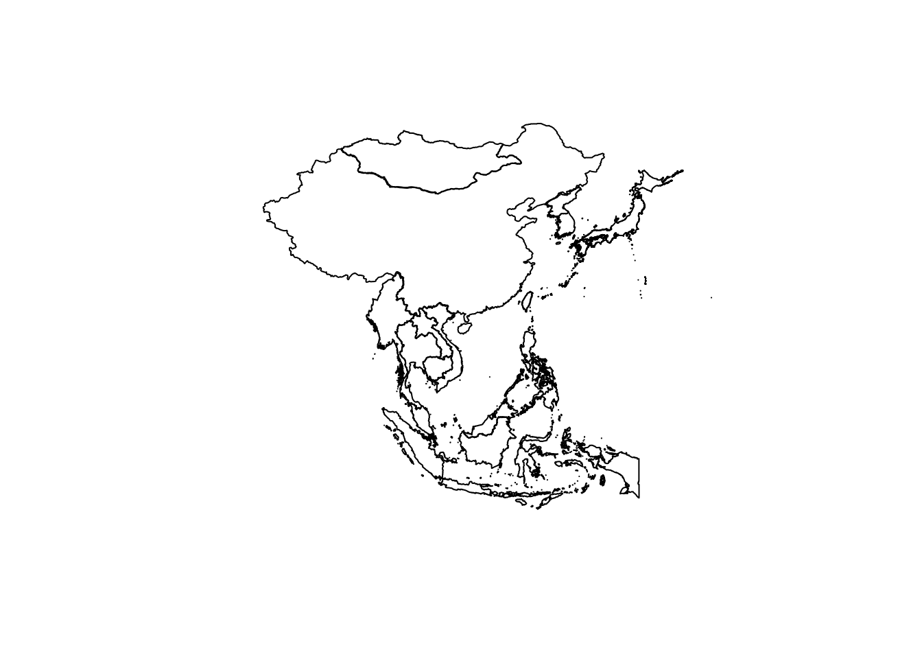

Research Area

Myanmar lies west of the specified longitude; therefore, replace China’s longitude value accordingly. Similarly, since Japan is located north of the specified latitude, replace China’s latitude value with that of Japan. Japan is also situated east of the specified longitude.

The research area includes a 3 km buffer. Given that 0.01 degrees correspond to approximately 1.11 km, appropriate adjustments should be made.

tmp <- em_boundary %>% st_bbox
tmp_xmin <- em_boundary %>% filter(shapeGroup == "MMR") %>% st_bbox
tmp_ymax <- em_boundary %>% filter(shapeGroup == "JPN") %>% st_bbox
tmp_xmax <- em_boundary %>% filter(shapeGroup == "JPN") %>% st_bbox
tmp_ymin <- em_boundary %>% filter(shapeGroup == "IDN") %>% st_bbox
tmp[[1]] <- tmp_xmin[[1]]
tmp[[4]] <- tmp_ymax[[4]]
tmp[[2]] <- tmp_ymin[[2]]
tmp[[3]] <- tmp_xmax[[3]]
tmp[1] <- tmp[1] - 0.03
tmp[2] <- tmp[2] - 0.03
tmp[3] <- tmp[3] + 0.03
tmp[4] <- tmp[4] + 0.03

Use st_as_sfc() %>% st_sf() if you only have geometry data and need to manually create an sf object.
st_as_sfc(x): Converts an object (like WKT, WKB, or a numeric matrix) into a simple feature geometry list-column (sfc).
st_sf(sfc_object): Wraps the sfc object in a simple feature (sf) data frame.

aoi <- tmp %>% st_as_sfc %>% st_sf
plot(aoi, graticule = TRUE, axes = TRUE)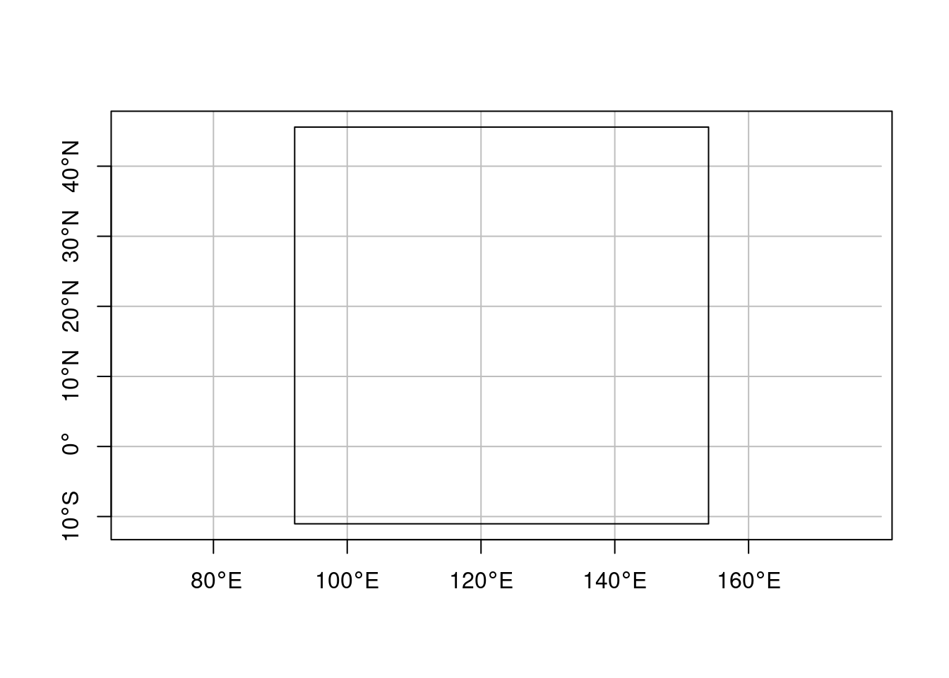

Area of Interest East and Southeast Asia

Mapping

Leaflet

dir_leaflet <- "figures/leaflet/"
m <- leaflet(aoi) %>% addTiles() %>% addPolygons(color = "blue", weight = 1, fillOpacity = 0.1)
filename <- paste0("aoi", ".html")
saveWidget(m, paste0(dir_leaflet, filename), selfcontained = TRUE)

leaflet(aoi) %>% addTiles() %>% addPolygons(color = "blue", weight = 1, fillOpacity = 0.1)

Area of interest

tmap

tmap_mode("view")
p <- tm_shape(aoi) + tm_borders(lwd = 2)
p

Area of interest

Climate Data

TerraClimate is a high-spatial resolution (4km) gridded dataset of monthly climate and hydroclimate for global land surfaces from 1958 to present ( TERRACLIMATE Dataset; Abatzoglou et al. (2018)).

In this research, monthly data for precipitation, temperature (max and min), climate water deficit, and potential and actual evapotranspiration provided in this database are used.

Importing Terraclimate data into R

NetCDF

esri explains that NetCDF (network Common Data Form) is a file format for storing multidimensional scientific data (variables) such as temperature, humidity, pressure, wind speed, and direction.

SpatRaster

Methods to create a SpatRaster. These objects can be created from scratch, from a filename, or from another object.

A SpatRaster represents a spatially referenced surface divided into three dimensional cells (rows, columns, and layers).

When a SpatRaster is created from one or more files, it does not load the cell (pixel) values into memory (RAM). It only reads the parameters that describe the geometry of the SpatRaster, such as the number of rows and columns and the coordinate reference system. The actual values will be read when needed.

Note that there are operating system level limitations to the number of files that can be opened simultaneously. Using a SpatRaster of very many files (e.g. 10,000) may cause R to crash when you use it in a computation. In situations like that you may need to split up the task or combine data into fewer (multi-layer) files. Also note that the GTiff format used for temporary files cannot store more than 65535 layers in a single file.

(Source: R documentation)

Precipitation

years <- seq(1958,2024)
ncpath <- "data/TerraClimate_data/"
ncname <- "TerraClimate_ppt_"

for (x in years){
    ncfname <- paste0(ncpath, ncname, x, ".nc")
    object <- rast(ncfname, subds = "ppt")
    assign(paste0("cl_ppt_", x), object)
}
plot(cl_ppt_1958[[1]])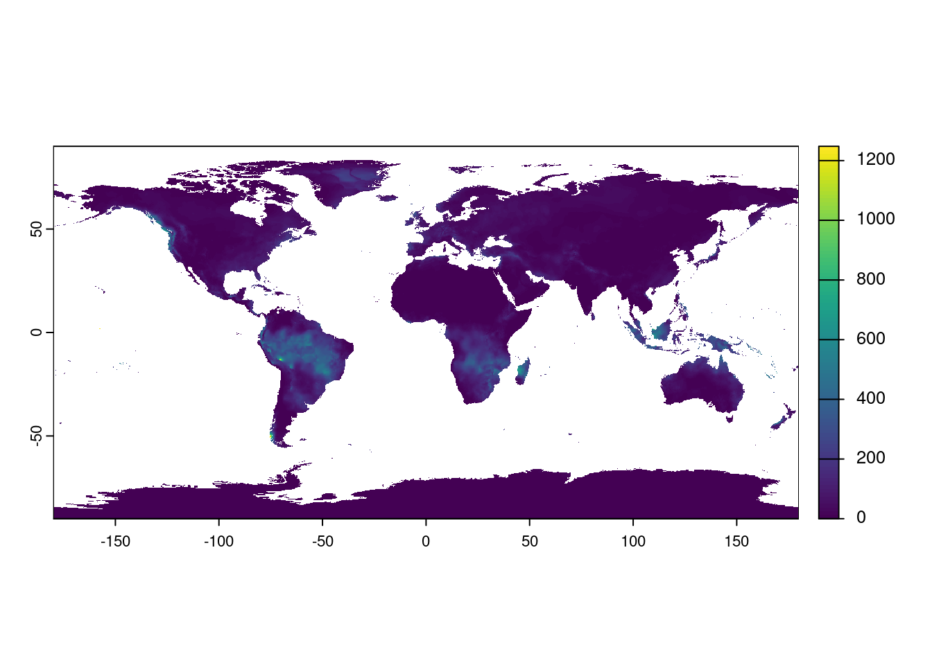

Cropping climate data by AOI

Crop monthly precipitation data by AOI and save it to tif format file.

ras_dir <- "data/raster/"

system.time(
    for (x in years) {
        fname <- get(paste0("cl_ppt_", x))
        object <- crop(fname, aoi)
        cname <- paste0("mon_cl_ppt_", x)
        c_object <- writeRaster(object,
                                filename = file.path(ras_dir, paste0(cname, ".tif")),
                                overwrite = TRUE)
        assign(cname, c_object)
    }
)

Mapping Precipitation

# load data into R
ras_dir <- "data/raster/"
for (x in years){
    ncfname <- paste0(ras_dir, "mon_cl_ppt_", x, ".tif")
    object <- rast(ncfname)
    assign(paste0("mon_cl_ppt_", x), object)
}

# Display
r <- mon_cl_ppt_1958[[1]]
r_pal <- colorNumeric(palette = "viridis", domain = values(r), na.color = "transparent")

leaflet() %>%
  addTiles() %>%  # Add base map
  addRasterImage(r, colors = r_pal, opacity = 0.8) %>%
  addLegend(pal = r_pal, values = values(r), title = "Raster Values")

Cropped precipitation distribution in January 1958

Creating annual rainfall object

Creating a multilayer object accommodating annual rainfalls from 1958 to 2024

# Annual rainfall
fhead <- "mon_cl_ppt_"
if (exists("a_rain")) {
    rm(a_rain)
}
for (x in years) {
    fname <- paste0(fhead, x)
    if (exists(fname)) {
        rd00 <- get(fname)
        rd01 <- app(rd00, sum) # calc() in the raster package
        names(rd01) <- x
        if (!exists("a_rain")) {
            a_rain <- rd01
        } else {
            a_rain <- c(a_rain, rd01)
        }
    } else {
        warning(paste0("The object does not exits: ", x))
    }
}

cat(src(a_rain), "\n")
# newcrs <- "+proj=longlat +datum=WGS84"
newcrs <- "EPSG:4326"
a_rain <- project(a_rain, newcrs)
a_rain <- writeRaster(a_rain,
    filename = file.path(
        ras_dir,
        "a_rain.tif"
    ), overwrite = TRUE
)

Mapping annual rainfall in 1958

Tmap

a_rain <- rast(file.path(ras_dir, "a_rain.tif"))
tmap_mode("view")
tm_shape(a_rain[[1]]) + tm_raster()

Leaflet

r_pal <- colorNumeric(palette = "viridis", domain = values(a_rain[[1]]), na.color = "transparent")

# for R in docker
# base_path <- "./data/raster"
# r <- raster(file.path(base_path, "ar_1958.gri"))

leaflet() %>%
    addTiles() %>% # Add base map
    addRasterImage(a_rain[[1]], colors = r_pal, opacity = 0.8) %>%
    addLegend(pal = r_pal, values = values(a_rain[[1]]),
              title = "Raster Values")

Importing other climate variables

max and min temperature, ppt, aat, soil moisture, and def

years <- seq(1958, 2024)
ncpath <- "data/TerraClimate_data/"
ncname <- "TerraClimate_"
variables <- c("aet", "def", "pet", "q", "tmax", "tmin")

for (var in variables) {
    for (ye in years) {
        ncfname <- paste0(ncpath, ncname, var, "_", ye, ".nc")
        object <- rast(ncfname,  subds = cli)
        assign(paste0("cl_", var, "_", ye), object)
    }
    printf("\n%s has been successfully imported.", var)
}

Cropping climate data by AOI.

for (var in variables) {
    for (ye in years) {
        fname <- paste0("cl_", var, "_", ye)
        fdata <- get(fname)
        object <- crop(fdata, aoi)
        cname <- paste0("mon_", fname)
        c_object <- writeRaster(object,
            filename = file.path(
                ras_dir,
                paste0(cname, ".tif")
            ),
            overwrite = TRUE
        )
        assign(cname, c_object)
    }
}

Remove unnecessary intermediate objects

rm(list = ls(pattern = "^cl_"))
rm(list = ls(pattern = "^mon_"))

Net Primary Production (NPP)

Estimation of Potential NPP

The Potential Net Primary Production (NPP) is estimated using Miami model, as presented in Lieth (1973)(Lieth (1973)).

\[ NPP(Temp, Precip) = min((\frac{a}{1+exp(b-c*Temp)}), (d(1-exp(e*(Precip))))) \]

Where \(Temp\) is the mean annual temperature (°C), \(Precip\) is the mean annual precipitation (mm/year),

The constants are empirically determined as: \[ \begin{align} a &= 3000 \\ b &= 1.315 \\ c &= 0.119 \\ e &= 0.000664 \\ \end{align} \]

This model estimates NPP as the minimum of two functions: one driven by temperature and the other by precipitation.

First of all, we create datasets of max and minimum annual temperatures from 1958 to 2024.

years <- seq(1958, 2024)
ras_dir <- "data/raster/"

for (var in c("tmax", "tmin")) {
    for (year in years) {
        fname <- paste0("mon_cl_", var, "_", year)
        file_name <- paste0(fname, ".tif")
        rasd <- rast(file.path(ras_dir, file_name))
        assign(fname, rasd)
    }
}

var <- "tmin"
fhead <- paste0("mon_cl_", var, "_")
objname <- paste0("a_", var)
if (exists(objname)) {
    rm(list = objname)
}
for (year in years) {
    fname <- paste0(fhead, year)
    if (exists(fname)) {
        rd00 <- get(fname)
        rd01 <- app(rd00, mean)
        names(rd01) <- year
        if (!exists(objname)) {
            assign(objname, rd01)
        } else {
            existing <- get(objname)
            combined <- c(existing, rd01)
            assign(objname, combined)
        }
    } else {
       warning(paste0("The object does not exits: ", year))
    }
    printf("%d is successfully imported\n", year)
}

vars <- c("tmax", "tmin")
for (var in vars) {
    fname <- paste0("a_", var)
    writeRaster(fname, filename = file.path( ras_dir, paste0(fname, ".tif")), overwrite = TRUE)
}
rm(list = ls(pattern = "^mon_"))

Now, we can compute mean annual temperature.

vars <- c("a_tmax", "a_tmin")
for (var in vars) {
    fdata <- rast(file.path(ras_dir, paste0(var, ".tif")))
    assign(var, fdata)
}

# Calculate mean max temperature and min temperature for each layer

a_tmean <- (a_tmin + a_tmax) / 2

writeRaster(a_tmean, filename = file.path( ras_dir, "a_tmean.tif"), overwrite = TRUE)

Finally, we can estimate NPP using the Miami model.

vars <- c("a_rain", "a_tmean")
for (var in vars) {
    fdata <- rast(file.path(ras_dir, paste0(var, ".tif")))
    assign(var, fdata)
}

fun_t <- function(x) {
    3000 / (1 + exp(1.315 - 0.119 * x))
}
fun_p <- function(x) {
    3000 * (1 - exp(-0.000664 * x))
}
npp_t <- app(a_tmean, fun_t)
npp_p <- app(a_rain, fun_p)
a_npp <- min(npp_t, npp_p)

writeRaster(npp_t, filename = file.path(ras_dir, "npp_t.tif"), overwrite = TRUE)
writeRaster(npp_p, filename = file.path(ras_dir, "npp_p.tif"), overwrite = TRUE)
writeRaster(a_npp, filename = file.path(ras_dir, "a_npp.tif"), overwrite = TRUE)

##### mean annual npp for all

a_npp <- rast(file.path(ras_dir, paste0("a_npp.tif")))
rmap <- subset(a_npp, 1)
max_val <- global(rmap, fun = "max", na.rm = TRUE)[[1]]
npp_legend <- c(0, 200, seq(500, 2500, by = 500), max_val)

tmap_mode("view")
p <- tm_shape(rmap) +
    tm_raster(col.scale = tm_scale(col = npp_legend, values = "brewer.bu_gn"))
p

NPP in 1958

References

Abatzoglou, J. T., S. Z. Dobrowski, S. A. Parks, and K. C. Hegewisch. 2018. TerraClimate, a high-resolution global dataset of monthly climate and climatic water balance from 1958–2015. Scientific Data 5:170191.

Boserup, E. 1965. The conditions of agricultural growth: The economics of agrarian change under population pressure. 3. pbk print. Allen & Unwin, London.

Fukui, H., and H. Fukui. 1993. Food and population in a Northeast Thai village. Univ. of Hawaii Press, Honolulu.

Kira, T. 2012. Geographical Distribution of Plants—A Reconsideration of Biological Nature. Shinju-sha, Tokyo.

Kono, Y., T. Sato, and I. Watanabe. 2012. Mechanisms of Agricultural Development in the Tropical Biosphere. Pages 257–282 The Potential of the Geosphere-Biosphere: The Survival Foundations of Tropical Societies. Kyoto University Press, Kyoto.

Lieth, H. 1973. Primary production: Terrestrial ecosystems. Human Ecology 1:303–332.

Moraga, P., and L. Baker. 2022, July. Rspatialdata: A collection of data sources and tutorials on downloading and visualising spatial data using R. F1000Research.

Scott, J. C. 2010. The Art of Not Being Governed: An Anarchist History of Upland Southeast Asia. Illustrated edition. Yale University Press, New Haven London.

Tanaka, K. 2010. Sustainable Agriculture as a Foundation for Livelihood in the East Asian Monsoon Region. Pages 185–209 Geosphere, Biosphere, Human Sphere: In Search of Sustainable Foundations for Human Survival. Kyoto University Press, Kyoto.